DIGITAL IMAGE INTERPOLATION
Image interpolation occurs in all digital photos at some stage — whether this be in bayer demosaicing or in photo enlargement. It happens anytime you resize or remap (distort) your image from one pixel grid to another. Image resizing is necessary when you need to increase or decrease the total number of pixels, whereas remapping can occur under a wider variety of scenarios: correcting for lens distortion, changing perspective, and rotating an image.

Even if the same image resize or remap is performed, the results can vary significantly depending on the interpolation algorithm. Itis only an approximation, therefore an image will always lose some quality each time interpolation is performed. This tutorial aims to provide a better understanding of how the results may vary — helping you to minimize any interpolation-induced losses in image quality.
CONCEPT
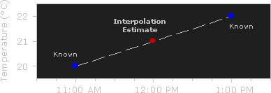
Interpolation works by using known data to estimate values at unknown points. For example: if you wanted to know the temperature at noon, but only measured it at 11AM and 1PM, you could estimate its value by performing a linear interpolation:
If you had an additional measurement at 11:30AM, you could see that the bulk of the temperature rise occurred before noon, and could use this additional data point to perform a quadratic interpolation:
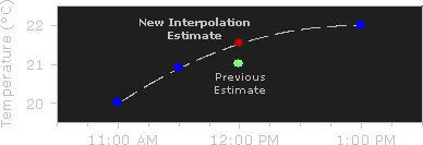
The more temperature measurements you have which are close to noon, the more sophisticated (and hopefully more accurate) your interpolation algorithm can be.
IMAGE RESIZE EXAMPLE
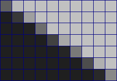
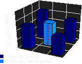
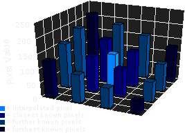
Image interpolation works in two directions, and tries to achieve a best approximation of a pixel's color and intensity based on the values at surrounding pixels. The following example illustrates how resizing / enlargement works:

→


Unlike air temperature fluctuations and the ideal gradient above, pixel values can change far more abruptly from one location to the next. As with the temperature example, the more you know about the surrounding pixels, the better the interpolation will become. Therefore results quickly deteriorate the more you stretch an image, and interpolation can never add detail to your image which is not already present.
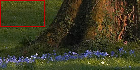
IMAGE ROTATION EXAMPLE
Interpolation also occurs each time you rotate or distort an image. The previous example was misleading because it is one which interpolators are particularly good at. This next example shows how image detail can be lost quite rapidly:
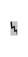
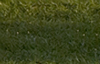
 Original
→
 45° Rotation
 90° Rotation
(Lossless)
 2 X 45°
Rotations
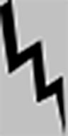
 6 X 15°
Rotations
The 90° rotation is lossless because no pixel ever has to be repositioned onto the border between two pixels (and therefore divided). Note how most of the detail is lost in just the first rotation, although the image continues to deteriorate with successive rotations. One should therefore avoid rotating your photos when possible; if an unleveled photo requires it, rotate no more than once.
The above results use what is called a "bicubic" algorithm, and show significant deterioration. Note the overall decrease in contrast evident by color becoming less intense, and how dark haloes are created around the light blue. The above results could be improved significantly, depending on the interpolation algorithm and subject matter.
TYPES OF INTERPOLATION ALGORITHMS
Common interpolation algorithms can be grouped into two categories: adaptive and non-adaptive. Adaptive methods change depending on what they are interpolating (sharp edges vs. smooth texture), whereas non-adaptive methods treat all pixels equally.
Non-adaptive algorithms include: nearest neighbor, bilinear, bicubic, spline, sinc, lanczos and others. Depending on their complexity, these use anywhere from 0 to 256 (or more) adjacent pixels when interpolating. The more adjacent pixels they include, the more accurate they can become, but this comes at the expense of much longer processing time. These algorithms can be used to both distort and resize a photo.
 Original
 Enlarged 250%
Adaptive algorithms include many proprietary algorithms in licensed software such as: Qimage, PhotoZoom Pro, Genuine Fractals and others. Many of these apply a different version of their algorithm (on a pixel-by-pixel basis) when they detect the presence of an edge — aiming to minimize unsightly interpolation artifacts in regions where they are most apparent. These algorithms are primarily designed to maximize artifact-free detail in enlarged photos, so some cannot be used to distort or rotate an image.
NEAREST NEIGHBOR INTERPOLATION
Nearest neighbor is the most basic and requires the least processing time of all the interpolation algorithms because it only considers one pixel — the closest one to the interpolated point. This has the effect of simply making each pixel bigger.
BILINEAR INTERPOLATION
Bilinear interpolation considers the closest 2x2 neighborhood of known pixel values surrounding the unknown pixel. It then takes a weighted average of these 4 pixels to arrive at its final interpolated value. This results in much smoother looking images than nearest neighbor.
The diagram to the left is for a case when all known pixel distances are equal, so the interpolated value is simply their sum divided by four.
BICUBIC INTERPOLATION
Bicubic goes one step beyond bilinear by considering the closest 4x4 neighborhood of known pixels — for a total of 16 pixels. Since these are at various distances from the unknown pixel, closer pixels are given a higher weighting in the calculation. Bicubic produces noticeably sharper images than the previous two methods, and is perhaps the ideal combination of processing time and output quality. For this reason it is a standard in many image editing programs (including Adobe Photoshop), printer drivers and in-camera interpolation.
HIGHER ORDER INTERPOLATION: SPLINE & SINC
There are many other interpolators which take more surrounding pixels into consideration, and are thus also much more computationally intensive. These algorithms include spline and sinc, and retain the most image information after an interpolation. They are therefore extremely useful when the image requires multiple rotations / distortions in separate steps. However, for single-step enlargements or rotations, these higher-order algorithms provide diminishing visual improvement as processing time is increased.
INTERPOLATION ARTIFACTS TO WATCH OUT FOR
All non-adaptive interpolators attempt to find an optimal balance between three undesirable artifacts: edge halos, blurring and aliasing.
 Original
400%
→
 Blurring
 Edge Halo
Even the most advanced non-adaptive interpolators always have to increase or decrease one of the above artifacts at the expense of the other two — therefore at least one will be visible. Also note how the edge halo is similar to the artifact produced by over sharpening with an unsharp mask, and improves the appearance of sharpness by increasing acutance.
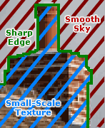
Adaptive interpolators may or may not produce the above artifacts, however they can also induce non-image textures or strange pixels at small-scales:
 Original
220%
→
 Adaptive Interpolation
On the other hand, some of these "artifacts" from adaptive interpolators may also be seen as benefits. Since the eye expects to see detail down to the smallest scales in fine-textured areas such as foliage, these patterns have been argued to trick the eye from a distance (for some subject matter).
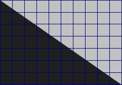
ANTI-ALIASING
Anti-aliasing is a process which attempts to minimize the appearance of aliased or jagged diagonal edges, termed "jaggies." These give text or images a rough digital appearance:
(With Aliasing)
(Without Aliasing)
Anti-aliasing removes these jaggies and gives the appearance of smoother edges and higher resolution. It works by taking into account how much an ideal edge overlaps adjacent pixels. The aliased edge simply rounds up or down with no intermediate value, whereas the anti-aliased edge gives a value proportional to how much of the edge was within each pixel:
 Perfect Diagonal
| Choose: | Aliased | Anti-Aliased |
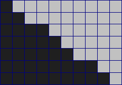 Resampled to Low Resolution
A major obstacle when enlarging an image is preventing the interpolator from inducing or exacerbating aliasing. Many adaptive interpolators detect the presence of edges and adjust to minimize aliasing while still retaining edge sharpness. Since an anti-aliased edge contains information about that edge's location at higher resolutions, it is also conceivable that a powerful adaptive (edge-detecting) interpolator could at least partially reconstruct this edge when enlarging.
NOTE ON OPTICAL vs. DIGITAL ZOOM
Many compact digital cameras can perform both an optical and a digital zoom. A camera performs an optical zoom by moving the zoom lens so that it increases the magnification of light before it even reaches the digital sensor. In contrast, a digital zoom degrades quality by simply interpolating the image — after it has been acquired at the sensor.

 10X Optical Zoom
 10X Digital Zoom
Even though the photo with digital zoom contains the same number of pixels, the detail is clearly far less than with optical zoom. Digital zoom should be almost entirely avoided, unless it helps to visualize a distant object on your camera's LCD preview screen. Alternatively, if you regularly shoot in JPEG and plan on cropping and enlarging the photo afterwards, digital zoom at least has the benefit of performing the interpolation before any compression artifacts set in. If you find you are needing digital zoom too frequently, purchase a teleconverter add-on, or better yet: a lens with a longer focal length.
For further reading, please visit more specific tutorials on:
Digital Photo Enlargement
Image Resizing for the Web and Email